Information entropy is in fact a more fundamental definition than our familiar Baltzmann entropy in stat mech.
When we use Boltzmann energy  , where W is the total number of microscopic states of the system with a given macroscopic state, we assume that all microscopic states has the same probability. This is true for most thermal systems. However, if the probability of each micro state is not the same, we have to modify the definition of entropy, then we have Gibbs entropy, which is equivalent to Shannon (information) entropy:
  , where
  is the probability of a state
  , and the sum takes over all
  ‘s. You can check that if all are equal, this definition goes back to Boltzmann entropy.
So we can have a ‘modern’ interpretation of thermal entropy: the amount of entropy means the amount of information we need to input into this system to determine its micro state for a given macro state. In other words, order means predictability, and for a specific state, the predictability means its probability. If a thermal system has a larger number of micro states, then each state would have smaller probability, which means we have a smaller chance to predict the right micro state, that’s why this system has a higher entropy.
A very useful lesson from thermal theory for us to understand order and disorder in information theory is: For two systems with the same macro state, the one with independent sub systems has higher entropy than the one with correlated sub systems. For example, ideal gas system has higher entropy than interacting gas system with the same micro state. We can use this intuition into information theory. For example, compare two pages of paper with the same number of letters on it. The letters on one page is totally random, while the other page is a well written article. So we say the letters on the first page are independent while the letters on the second page have some correlations with each other. To determine the micro structure of the first page, we have to put in the information of each letter, with probability  for each one. To determine the micro structure of the second page, we only need to put in the information of each word, with the probability larger than
  , where n is the number of letters in the word, since we know that there are some combination of letters which are definitely not a word. So now you can calculate the probability of each micro state, the second should be larger than the first. So we say the second page is more ‘predictable’, and the information comes from correlation. It’s interesting that we have just interpreted information entropy by using thermal entropy, for smaller probability of a micro state means larger number of micro states.
But there are 2 cases in which we can only use information entropy. One is, as I mentioned, when the probability of each micro state is not the same; Another one is non-equilibrium process. I am not familiar with either of them. Does any one know any examples of these cases?
The following is Lightsaber’s explanation of entropy in non-equilibrium process:
Let me start with non-equilibrium situations. In my lecture, I mentioned that “Information is …… boundary condition.” Many thought that “boundary condition” was a phrase I randomly picked, it’s not. Actually, I was referring to the non-equilibrium cases. Non-equilibrium is featured by non-uniform distribution and time-variance. By possessing the information of its spatial distribution, the entropy of the system is reduced. When equilibrium is established, all the information become no longer valid, and the entropy increases. That is why the establishment of equilibrium is always entropy-increasing. This piece of information could be valid only at a particular time, or be valid during the entire time interval we study. In the former case, it’s an “initial value condition” in PDE language, but it’s but a boundary condition in time domain anyway.
Starting from the simplest example in non-equilibrium thermodynamics: diffusion. If we connect a full bottle of nitrogen dioxide (bottle A) and a full bottle of air (bottle B) with a glass tube, we can see the red color gradually propagates, until the gas in both bottle has the same color. This is a entropy-increasing process. At the very beginning, we do know (know = possess a piece of valid information) that there’s neither air in A nor air in B. With the knowledge, the entropy is relatively low. In the language of probability theory as Shannon used, the probability of (an infinitesimal domain) in bottle A being filled with NO2 is 1, while it is 0 in bottle B. After the establishment of equilibrium, this piece of information become completely invalid, and the entropy is larger.
However, how can we describe the dynamical process (the formal term is “transport process” I think) between the start and the equilibrium? Can we use information theory to process it? I believe so.
In my PERSONAL opinion which hasn’t appeared on any reference material I’ve read so far, the introduction of fuzzy mathematics will be a possible way to solve it. Darthmaverick is an outstanding expert in this area, but I can discuss to the best of my knowledge. We can define a “membership function of validity” for any piece of information, which is dependent on time. This membership function can be determined as “The probability that the piece of information is true”. For example, for the statement “Bottle A is full of NO2 without air”, we can define the membership function as “P(an infinitesimal domain is filled with NO2)-P(an infinitesimal domain is filled with air)”. At the starting of transpotation, this membership function is 1, and it becomes 0 eventually. It can be proven (though I haven’t done it myself) that this membership function could be constructed to be proportional to the “entropy decreasing capability” of the corresponding information, as in the example above.
The utilization of this measure is still to be explored. After all, I come up with this combination of non-equilibrium thermodynamics, information theory and fuzzy mathematics independently, and it’s expected that some original work can be done following this direction.
That’s all for now, thank you.
As to the cases in which “the probability of each micro state is not the same”, intuition told me that it’s EQUIVALENT to the non-equilibrium cases, or uniquely corresponds to one. I wish I could prove it mathematically, but I cannot do it in a rigorous way. Possibly it’s wrong anyway.
One of the possible way of proving it is to consider the symmetry of the system. The unsymmetry of different microstates vs the broken symmetry the macroscopic system, what’s the connection?
Plus, according to LOT2, a closed system tends to maximize its entropy. Can a system reach the GLOBAL maximum of entropy without eliminating the unsymmetry among microstates?
I wish I could find an example in which symmetry among microstates is essentially and permanently broken. If it exists, and it can be stablized given time, my hypothesis in the 1st paragraph is wrong.
Then CoolPro asked an interesting question (in Chinese):
我想问问,ABCD四个球在正方形四顶角上
状态1,A朝东,B朝西,C朝南,D朝北。
状态2,B朝东,C朝西,D朝南,A朝北。
如果这时候算W,那上边两个状态是否可以算作相同的地位,从而总共算两个状态?即W=1+1+····
可是实际上,东西南北这个方位信息是我们给的,我们如果不给这个信息的话,这两个状态就是一个状态。
也就是说,给的信息越多,状态就越多,最终决定状态是否相同的是信息,但是信息的量,是怎么掌控的?我可以无限制地加信息,那熵就会无限制地减小。那么一个确定的系统的熵是可以无限多个的。
这是否跟我们的“事实”相违?一个确定的系统,却有不同的指标·····感觉很矛盾,估计只能在人类意识涉及到的地方才存在了
My answer is:
你说得不错,熵的确定确实依赖于我们给定的信息。我的印象是,在解决热学体系问题时,如何确定熵确实是一个很不简单的问题。确定一个系统的熵之前,我们需要定义这个宏观系统,即给定这个系统的一套完整独立的宏观参数,比如温度、能量、体积等,也包括LS提到的那些边界条件。在确定了这些信息之后,我们只需要问,还需要多少微观状态的信息才能把这个系统唯一地确定下来,这就是熵。但这里就有一个问题,也是你问到的问题:什么叫“唯一”?我怎么知道两个微观态是不是同一个?原则上,我们永远也不知道,因为一个体系的自由度多少取决于我们看这个系统所用的尺度,尺度越小,分辨越精细,自由度也就越多。同样两个状态,在大尺度上看可能是一样的,但在小尺度上看就有区别。所以可以理解,对同一个客观系统,当我们用的尺度越大时,算出来的熵越小,反之,熵越大。当然,“尺度”这个概念可以再抽象一下,变成我们关心的自由度和不关心的自由度。在你的例子里,第一种情况我们关心方位,尺度小,所以熵大,第二种情况不关心方位,尺度大,所以熵小。还有一个典型情况就是粒子全同性问题,全同粒子体系是比可区分粒子体系的熵小的。
所以说,系统是由信息确定的,即便我们面对的是同一个客观系统,只要我们预设的信息不一样,系统就不一样。这样做的有效性在于:我们通常只关心一个系统在演化中的熵变,而不关心它的绝对熵值,在不涉及系统自由度的动力学变化的时候,不同定义的熵只相差一个常数,而演化之间的熵变是唯一确定的。这可以类比量子场论中的重整化:当我们在不同程度上忽略更精细的结构时(比如加上一个动量截断),算出来的物理量也相差一个常数(尽管这个常数依赖于截断),但不会改变物理体系的变化方式(即参数在不同能标间的跑动以及由此算出来的观测量值)。
当然,并不是所有情况都是安全的。当体系的自由度发生动力学变化时,以前所假设的“模糊”自由度下所定义的熵就失效了。用场论的语言说,就是有效场论失效。比如说一团气体,我们先用分子做自由度,分子内部的不同结构在我们眼里对应同一个态。但后来由于能量升高,分子内部的结构变化开始影响到分子之间的相互作用,我们就不得不把分子自身变化的熵变计算到总熵里面,也就是说,这个时候可能就需要取原子或者原子团做自由度,把不同分子结构当成不同状态了。当然一个原则上一样方向却相反的例子是粒子全同性,我们从前以为粒子是可区分的,结果在计算气体混合熵的时候出现Gibbs样谬,才发现粒子应该是全同的,我们区分得过于精细,而这并非真实的状况。至于你提到的四个球的问题,是个很好的例子。如果我们把它想象成一种分子结构,当这个分子在三维空间里自由悬浮的时候,两个状态可以通过旋转变成一样,所以它们是同一种状态;而当这个分子被固定在二维平面上的时候,他们就是不同状态。所以说,怎么确定自由度还要看我们的物理体系会受到那些因素的影响,并不是那么地随意。
一个附带问题:压缩信息时熵怎么变化?
答:无损压缩熵不变,有损压缩么。。。如果按照“不同自由度,不同系统”的说法,有损压缩后自由度减少,由此算得的熵应该是更小,但显然不合理,因为比较两个不同方式定义的系统是没有意义的。所以,我们应该拿同样的自由度来比较,都用压缩前的自由度,有损压缩相当于是增加了被压缩的那部分状态的可能状态数,所以熵应该更大。
Another piece of LS’ comments:
A microstate is a specific, detailed configuration that includes the state of all the particles inside. For an N-particle system, it’s one single point in the 6N-dimensional phase space. For example, for a system described by canonical ensemble, its equilibrium macrostate is consist of numerous microstates, EACH OF WHICH obeys Gibbs distribution (cuz each microstate contains a complete set of information about all the particles and thus has its OWN distribution), and has the same probability as each other. If we change the parameters (like T), the equilibrium state will be consist of another set of microstates, but each of them will still obey Gibbs distribution and will has the same probability as each other.
My response:
To my knowledge, Gibbs distribution (or more commonly called ‘Gibbs measure’, or ‘Boltzmann distribution’) means the probability of a microstate of a system, not the distribution of the particles in this system. If this is not GL means, that’s fine, we don’t need to debate on terminologies. But I do have some more comments. The phase space you mentioned is for microcanonical ensembles, in which the density of states is a constant, which means all microstates, no matter what macrostates it correspond to, have the same probability. This is true for microcanonical ensembles (or isolated systems), but not for canonical ensembles, which is exactly described by Gibbs measure. In the phase space of a canonical ensemble, the density of a certain microstate is not a constant, it can repeat for many times, and the density or probability of the microstate is proportional to the number of microstates of the reservoir which ‘coexist’ with it. When you consider this and do the calculation, you get the Gibbs measure.
We should distinguish ensemble language and distribution language. The former one is only interested in microstates of the whole system. It is so abstract that it never cares about what kind of system it is or the fate of a single particle in it, while this fate or distribution probability of a single particle is just the essential focus of the distribution language, and it’s result varies with the types of systems(classical, quantum, interacting or not, etc. ). And further, a given microstate in ensemble language has no ‘probability distribution’, cuz it’s totally determined, the so-called distribution is just a description of this state, and it can be way off the Boltzmann distribution, eg, some higher energy level may have more particles than some lower energy level. Some of us may confuse ‘Boltzmann distribution’ in ensenble language with that in distribution language. They have exactly the same mathematical form, but have very different meanings: one is for microstates of a system ensemble, one is for particles in a single system. Why they have the same form is just a coincidence, because ensembles are defined as classical and independent with each other, which is the same property of the particles in a classical non-interacting thermal system. But see, we have other kinds of thermal systems, eg, quantum boson or fermion system, and they do not obey Boltzmann distribution.

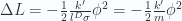
![L=\sum_i\frac{1}{2}[m\dot{q}_i^2-k(q_i-q_{i+1})^2]](https://s0.wp.com/latex.php?latex=L%3D%5Csum_i%5Cfrac%7B1%7D%7B2%7D%5Bm%5Cdot%7Bq%7D_i%5E2-k%28q_i-q_%7Bi%2B1%7D%29%5E2%5D&bg=fafcff&fg=2a2a2a&s=0&c=20201002)

![L=\lim_{l,m\to0}\int \frac{d^Dx}{l^D}\frac{1}{2}\left[m\dot{q}^2-kl^2(\partial_xq)^2\right]](https://s0.wp.com/latex.php?latex=L%3D%5Clim_%7Bl%2Cm%5Cto0%7D%5Cint+%5Cfrac%7Bd%5EDx%7D%7Bl%5ED%7D%5Cfrac%7B1%7D%7B2%7D%5Cleft%5Bm%5Cdot%7Bq%7D%5E2-kl%5E2%28%5Cpartial_xq%29%5E2%5Cright%5D&bg=fafcff&fg=2a2a2a&s=0&c=20201002)


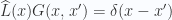
 is a linear differential operator.

 as a boundary condition that
  . This gives us the retarded Green’s functions. In RQM, the boundary condition becomes
  for
for  and
and 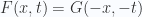 for
for  , where
  is the on-shell Green’s function without this time-ordered condition.
  is just the Feynman propagator.
 are indices for all internal degrees of freedom.
  are a complete set of states.
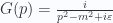

 is a matrix carrying spinor indices.
 is the polarization basis and
  is the ‘coordinate’ on this direction which is a pure number. To calculate the propagator, we take

 is gauge dependent for massless vector field so we see that the propagator is also gauge dependent.
 , 1 faithful but reducible rep of
 Poincare group
 . In particle physics, the role of representations is even more obvious: the nature has only one fundamental physics law, which means the groups that describe all the matters in the universe are the same, but why are there so many different species of fundamental particles with different spins and interactions? They are distinguished by different representations. Different spins and momenta are distinguished by rep’s of Poincare group, different interactions are distinguished by rep’s of gauge groups.
 and
and  are equivalent both as Lie algebras and groups (ie., they are isomorphic); While
  and
and  have the same algebra, they are different groups (
 , where
  means an action of
  . So if you stretch a quirk-antiquirk pair, the energy reserved in a unit length is
  , unlike QCD, it is less than the energy required for producing another quirk-antiquirk pair, so the string will never broken. It can be stretched to macro scale, depending on the cutoff. Because of the string, this pair can oscillate like a spring. This gives the quirk very rich phenomenology. The two talks focused on the detection signal of quirks, they argued about different life time of the string before it annihilates and the stuff shaken off during the oscillation.
 is introduced to form a 5 dimensional operator, whose UV completion is the propagator of a massive U(1) charged fermion
  . The UV completion allows only one type of quark coupled to
  . The generated mass are very close to the real values, by varying the couplings only between 0.3 and 3. This is the most beautiful part of the model.
 , which gives no hope to see them at LHC. But the constrain for a scalar field for downtype mass is
  .
. ,
,  ,
,  is model dependent, ie., take a particular model with undetermined parameter and calculate the expected observational curve and fit with the data. This talk provided a way to draw the parameters directly from data. The only assumption is RW metric and GR. From the general Friedman equation, we can express the coordinate distance and it’s first and second derivatives (wrt z) with those parameters. By analyzing the distance-redshift curve directly, we can fit the parameters. In order to determine w, which can vary with z, we need to construct another parameter called “dark energy indicator” s, which is 0 for w=-1. The fitted s with supernovae data is 0 for z<1, but when z goes close to 1, there is a bump. It’s still unclear whether this bump is caused by systematics or it has any physical meaning.